P&L with AI: build one from a trial balance

What you’ll end up with

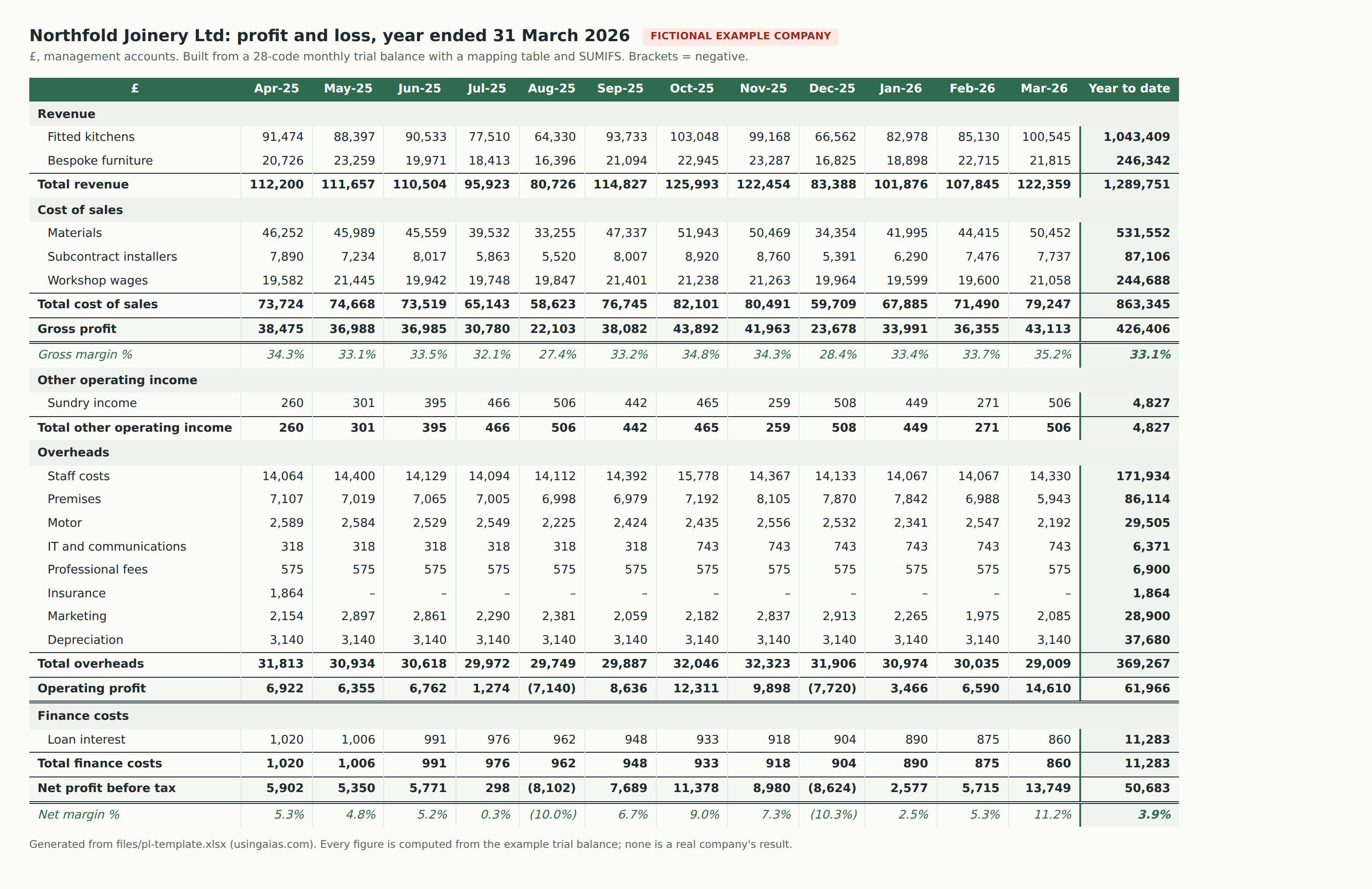
A monthly management P&L in Excel that rebuilds itself from a trial balance export. You decide once which P&L line each nominal code belongs to. After that, a lookup column and SUMIFS do the work every month, and three checks prove the result ties back to the TB.

The split of work is simple. AI proposes the mapping from codes and names only, writes the formulas and drafts the commentary. Excel does all the arithmetic. You make the judgement calls and sign it off.

Before you start

Everything below uses Northfold Joinery Ltd, a fictional fitted-kitchen and bespoke-furniture maker. It does not exist: the trial balance was generated for this guide to look like a UK joinery SME, with seasonal sales, a fixed workshop payroll, 2025-26 employer NI rates and quarterly VAT. Year ended 31 March 2026, 28 nominal codes (21 P&L, 7 balance sheet).

The workbook, the chart and the downloads on this page show the example’s tables, so the steps below give you the numbers to check against rather than repeating them.

Steps

1. Get the trial balance as monthly movements

Export 12 months from your accounting software with nominal code, account name and one column per month. You want movements (what happened in each month), not balances. If your software only gives year-to-date balances, add a sheet that takes each month minus the month before, and keep the first month as it is. Debits positive, credits negative.

Checkpoint: each month column nets to 0.00. The example has 28 codes across 12 months (Apr-25 to Mar-26) and every column balances.

2. Strip it down before AI sees anything

For the mapping you only need two columns: code and account name. Copy them to a new sheet. No amounts, no customer or staff names. If an account name contains a person’s name (some ledgers have “Director’s loan: J Smith”), rename it to something neutral like “Director’s loan account” first.

It feels fussy. It isn’t. The mapping only needs to know what an account is called, never what’s in it.

Checkpoint: a two-column list of 28 rows: codes and names, nothing else.

3. Ask AI to propose the mapping

Give it a fixed list of P&L lines, which stops it inventing lines, and ask it to flag ambiguity, which stops it hiding its guesses.

I'm building a management-accounts P&L in Excel for a UK joinery company (fitted kitchens and bespoke furniture).

Below is the chart of accounts: nominal code and account name only, no amounts.

Map every code to exactly one P&L line from this list, and give its section:
- Revenue: Fitted kitchens, Bespoke furniture
- Cost of sales: Materials, Subcontract installers, Workshop wages
- Other operating income: Sundry income
- Overheads: Staff costs, Premises, Motor, IT and communications, Professional fees, Insurance, Marketing, Depreciation
- Finance costs: Loan interest
- Balance sheet: any code that isn't income or expense

Return a table with four columns: Nominal code | Account name | P&L line | Section. One row per code, in code order.
If a code could reasonably go in two places, put your best choice and add a note underneath saying why it's ambiguous. Don't invent codes.

[paste the code and name columns here]

Then read every row. Yes, even the obvious ones. This is the one place where judgement goes in.

Northfold has three judgement calls: sundry income (4900) as revenue or other income; workshop wages (5200) as cost of sales or staff costs; employer’s NI and pension (7006, 7010) split between direct and office staff. We put sundry income below gross profit, workshop wages in cost of sales and all NI and pension in overheads. Any of these is defensible. What matters is that you choose once and keep it, because a P&L that changes shape every month is useless for comparison.

Checkpoint: a table of 28 rows, 7 of them Balance sheet, with notes on the judgement calls.

4. Set up three sheets: TB, Mapping, P&L

Paste the TB with codes in column A and months in C to N. Paste the reviewed mapping onto a Mapping sheet. Then add two helper columns to the TB that look each code up: the P&L line in P and the section in Q. Ask AI for the lookup if you don’t want to write it.

In Excel, on a sheet called TB, column A holds nominal codes (numbers) from row 2 down. A sheet called Mapping has code in A, account name in B, P&L line in C and section in D, rows 2 to 500.
Write a formula for TB!P2 that returns the P&L line for the code in A2, returns "UNMAPPED" if the code isn't on Mapping, and returns blank if A2 is empty. Then the same for the section in Q2. Use VLOOKUP or INDEX/MATCH so it works in older Excel. Explain each part in one line.

You should get something like this for the P&L line:

=IF($A2="","",IFERROR(VLOOKUP($A2,Mapping!$A$2:$D$500,3,FALSE),"UNMAPPED"))

Checkpoint: the formula is filled down to row 500, so next year’s new codes are caught, and filtering column P shows no row saying UNMAPPED.

5. Build the P&L with SUMIFS

Type your P&L line names in column A exactly as they appear on the Mapping sheet. Each number is a SUMIFS over the TB month column, matching the line name. Income lines get a minus sign in front, because credits are negative in the TB and you want revenue to show as a positive number.

My P&L sheet has line names in column A (for example "Fitted kitchens") and months across B to M. The TB sheet has monthly movements in C to N (debits positive, credits negative) and the P&L line for each row in column P, rows 2 to 500.
Write the formula for B6 that sums the April column of TB for the line named in A6. Income lines should show as positive, so flip the sign for those. Make the references lock correctly so I can copy it across 12 months and down every line.

For an income line it should look like this:

=-SUMIFS(TB!C$2:C$500,TB!$P$2:$P$500,$A6)

Checkpoint: April revenue on the example is £112,200 and full-year revenue £1,289,751. If it shows as a negative number, the sign flip is missing.

6. Or do steps 4 and 5 with Copilot in Excel

If your organisation has Copilot in Excel, open the workbook with the TB and Mapping sheets already in place and ask it to add the columns and formulas. If you don’t see Copilot, it may not be in your Microsoft 365 subscription or may not be available under your organisation’s settings.

On the TB sheet, add a column called P&L line that looks up each nominal code in column A on the Mapping sheet and returns the P&L line, or UNMAPPED if it isn't there. Then on the P&L sheet, fill B6:M28 with SUMIFS formulas that total the TB month columns by the line name in column A.

Read every formula it writes: click a cell and read the formula bar.

Checkpoint: the same numbers as step 5. If Copilot typed values instead of formulas, undo and ask again for formulas.

7. Add subtotals, gross profit and margins

Add a total for each section, then gross profit (revenue minus cost of sales), gross margin % (gross profit ÷ revenue, wrapped in IFERROR so a month with no revenue doesn’t show an error), operating profit (gross profit plus other operating income, minus overheads), finance costs and net profit before tax. A year-to-date column is just a SUM across the 12 months.

Checkpoint: full year on the example: gross profit £426,406, gross margin 33.1%, overheads £369,267, operating profit £61,966, net profit before tax £50,683 (3.9% of revenue). Gross margin runs from 27.4% (Aug-25) to 35.2% (Mar-26).

8. Add a month and year-to-date view

Put month numbers 1 to 12 above the P&L columns and a month selector on a new sheet. The month column is INDEX on the selected month; year to date is SUMPRODUCT of the months up to and including it.

=SUMPRODUCT(('P&L'!$B$3:$M$3<=$B$1)*'P&L'!$B8:$M8)

Checkpoint: select month 6 (Sep-25) on the example: revenue £114,827 for the month and £625,836 year to date; net profit £7,689 for the month and £16,908 year to date.

9. Build the checks, then make them pass

Three formula checks on their own sheet, which you look at before anything goes out:

1. The TB nets to zero in every month.
2. No code is UNMAPPED.
3. P&L net profit plus the TB’s total for the non-balance-sheet codes equals zero.

Add a fourth that flags gross margin outside the range you’d expect. Check 3 is the one that earns its place: it’s the only one that proves the P&L ties to the TB rather than just looking plausible.

Checkpoint: all say OK on the example. Then change one mapping row and watch them fail. A check you’ve never seen fail is a check you’re only hoping works.

10. Use AI to review the build and draft the words

Two last prompts. The first reviews your formulas without any data.

Here are the formulas from my P&L workbook (no data). Act as a reviewer who has closed a lot of month-ends. List anything that would silently give the wrong answer: ranges that won't extend, sign errors, text matches that could fail, hard-coded numbers. Be specific about cell references.

[paste formulas: use Formulas > Show Formulas, then copy]

The second drafts commentary from the summary figures you choose to give it, and only the reasons you supply. On real data, use your organisation’s approved tool for this step. The figures below are the fictional example’s.

Draft four short paragraphs of commentary for a monthly P&L, for the owner of a small joinery business. Plain English, no jargon, no adjectives like 'strong' or 'robust'.
Use only the figures and reasons I give you. If a variance needs a reason I haven't given, write [REASON NEEDED] instead of guessing.

Year to March 2026: revenue £1,289,751, gross profit £426,406 (33.1%), overheads £369,267, net profit before tax £50,683 (3.9%).
Losses in August (-£8,102) and December (-£8,624). Reason: revenue fell to £80,726 and £83,388 while workshop wages stayed around £19,847 a month.
New quoting software from October (£425 a month).

Check every figure in the draft against the sheet before it goes anywhere.

Checkpoint: the commentary explains the August and December losses with the reason you gave and leaves [REASON NEEDED] where you gave none. If it gives a reason you never provided, delete it.

Common mistakes

• Income showing as negative. A TB holds income as credits, so a plain SUMIFS returns negative revenue: -£1,289,751 on the example. Put a minus in front of the SUMIFS on income lines only, and say which sign convention you use in every prompt.
• A new code that isn’t mapped. Northfold started paying for quoting software in October on a new code, 7504. A mapping built from April’s TB doesn’t have it, so its £2,550 drops out: IT costs show £318.40 in October instead of £743.40, and net profit is overstated at £53,233. Check 2 shows one unmapped code and check 3 is out by £2,550.00. Fill the lookup down to row 500 and run the UNMAPPED check every month.
• Line names that nearly match. If one mapping row says “Premises “ with a trailing space, SUMIFS no longer matches it. On the example that drops light, heat and power: premises falls to £62,860 from £86,114. Nothing shows as UNMAPPED, because the code is mapped, so only check 3 catches it (out by £23,253.56). Put a data-validation list on the Mapping sheet’s line column, fed from the P&L’s line names, and keep the tie-back check.
• Year-to-date balances treated as monthly movements. Many systems export a trial balance as balances at a date. Summed across 12 columns, every line is massively overstated. Difference the columns first, then check a couple of lines against the system’s own monthly P&L.
• Annual costs posted in one month. Northfold’s insurance (£1,864) hits April only, and its business rates (£11,860) are billed in 10 instalments, April to January, so February and March carry none. The P&L is arithmetically right and still misleading month to month. Spread them with prepayments: £155.33 a month for insurance and £988.33 a month for rates on the example. That’s a journal in the ledger, not something a template can do for you.
• Accruals that don’t reverse. Northfold accrues its year-end accountancy fee at £575 a month, and when last year’s invoice arrived in December it was posted against the accruals account, so the P&L stayed smooth. Posted straight to the accountancy fees code, December would have taken the full invoice on top of the accrual. Ask of every lumpy line: is this the cost of this month, or the bill for another one?
• Leading zeros lost. Open a CSV in Excel and code 0051 becomes 51. If your mapping stores codes as text (“0051”), nothing matches. Keep codes as numbers in both sheets with a 0000 number format (the template does), or import the code column as Text in both.
• Letting AI do the sums. Paste a TB into a chat and ask for a P&L, and you’ll get a tidy table. Some totals may be wrong, and you can’t see how it got them. If a number didn’t come out of a formula, it doesn’t go in the pack.

When to keep AI out of it

Three things stay with you. The arithmetic, always: that’s Excel’s job. The mapping judgement itself: AI proposes, you decide, and calls like Northfold’s workshop wages or sundry income are yours to make and keep. And real figures or client data in a tool your organisation hasn’t approved.

Once the mapping exists, a new month is an export, a paste and a look at the checks. You can see every formula and explain it to anyone who asks.